Controlling Superposition
Introduction
In line with the first claim of Zoom In: An Introduction to Circuits, we consider features, mediated as directions, to be the fundamental of expression for neural networks. That is, directions in the latent spaces of neural networks are the units by which neural networks form their representations. I am not entirely convinced by this vision, some speculations I have come from the Polytope Lens, however, for the simplicity let us adopt this view.
Since neural networks store these representations in finite-dimensional vector spaces, it immediately becomes clear that the number of
Independent features can be extracted linearly from neural networks. Indeed, suppose that the latent space of a neural network has $n$ dimensions. If $\{\mathbf{v}_1,\dots,\mathbf{v}_n\}$ is our basis of features, then the $i^\text{th}$ feature of a representation $\mathbf{x}\in\mathbb{R}^n$ can be extracted as $$\mathbf{e}_i^\top\begin{pmatrix}\vert&&\vert\\\mathbf{v}_1&\dots&\mathbf{v}_n\\\vert&&\vert\end{pmatrix}^{-1}\mathbf{x},$$where $\mathbf{e}_i$ is the $i^\text{th}$ basis vector.
Since neural networks empirically demonstrate a capacity to utilises many more features than they have dimensions, they must not be relying on independent features. If it were the case that neural networks were using solely independent features, then interpretability would be a relatively easy task, since one would just have to search for an $n$-dimensional basis of features from which to reconstruct the model's behaviour. Therefore, there must be more to the story, and indeed there is due to the fact that neural networks are not
What are the additional capabilities that non-linearities offer?
To understand these capabilities we can focus on the ReLU. Geometrically, the ReLU non-linearity can be thought of as folding the representations in the space on which it is applied. Meaning previously non-independent features, that is features that are not completely orthogonal, can be disentangled by the non-linearity; allowing for the subsequent linear layer to extract the features of interest. Moreover, the ReLU non-linearity has a thresholding capacity, namely it can eliminate low-level noise in the reconstruction process of representations in terms of the features, see
These capabilities mean that neural networks can store features that are not strictly independent, but have some interference. Although this leniency may seem insignificant, it is exponentially significant thanks to the Johnson-Lindenstrauss lemma; which says that by allowing some fixed small amount of overlap between the directions, we can store exponentially many of the features.
The extent to which a neural network can utilise the the Johnson-Lindenstrauss lemma depends on the extent to which the neural network can utilise its non-linearities to minimise the effect of the interference. The more features the model tries to store with some interference the greater the pressure on the non-linearity. Similarly, there will be greater pressure on the non-linearity if the pertinent features of the tasks are highly correlated.
Therefore, the neural network training process can be interpreted as the model identifying what and how many features it can store with sufficiently low levels of interference. For instance, if the model identifies features that are rarely active simultaneously, it can store them with greater interference.
Of course, this is a speculative discussion on how neural networks behave, however, there is significant empirical evidence that this is a large part of the neural network story, evidenced by the success of sparse autoencoders at extracting features. Thus idea is summarised as the superposition hypothesis, and understanding the extent to which the superposition hypothesis holds is a fascinating open question. Making progress toward this question is important since it has ramifications for how we reason about the behaviours models. For instance, superposition is often used as an explanation for polysemantic neurons - which are neurons active on seemingly disjoint concepts. Polysemantic neurons are troublesome for work in mechanistic interpretability as they inhibit attempts to efficiently explain the behaviour of a neural network through analysing the behaviour of its internal components. If we can understand what mediates the extent to which models utilise superposition, we may be able to work toward developing more interpretable models - from the perspective of mechanistic interpretability at least.
Although superposition can explain part of the story as to why neural networks can seemingly utilise many more features than they have neurons, there are other possible explanations of this phenomena. For instance, compositionality provides an alternative mechanism which is actually argued to be at odds with superposition. Suggesting that the extent to which models use superposition exists on a spectrum. In some cases there may be a relatively small set of simple features that are highly expressive, meaning that compositionality can be effectively leveraged. On the other hand, features may be plentiful and sparse, in which case the model would benefit from storing features in superposition.
In this work, we investigate the superposition portion of the story by exploiting its reliance on the non-linearity, to try and work toward an understanding of how much a model relies on superposition.
Toy Models
Basic Setup
Let us start with the toy model set up of Toy Models of Superposition. We want to intervene on the non-linearity of these models and explore the subsequent effects on superposition. Thankfully, the ReLU provides an elegant way of doing this. By changing the slope of the negative component from $0$ to $1$, we can go from fully non-linear to linear, with intermediate slopes providing a varying level of non-linearity. These deformed activation functions are colloquially known as leaky ReLU activation functions, whose parameter governs the slope of the negative component.
Doing this we observe that we gradually reduce the extent to which the model is superimposing features. With
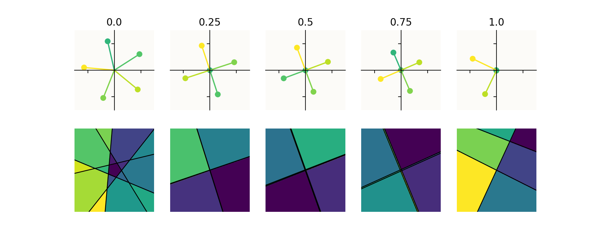
This supports our hypothesis that the non-linearity is crucial for controlling the extent to which neural networks can superimpose features.
In the second row of the figure we observe the effects this has on the partitioning of the latent space of the neural networks, which is relevant for the previously mentioned Polytope lens. On each partition the neural network is an affine operation. Since the partitions are inherently related to the non-linearities of the model, they can provide some valuable insight. Indeed, we observe that the partitions are concentrated around the features when they are in superposition, whereas they disappear when superposition fails; further supporting that the presence of the non-linearity is crucial for superposition.
Extended Setup
In the above setup we have implicitly set values for the importance of the features and set the size of the latent dimension to two, allowing for clear visualisations. Here we explore further the dependencies of the above results on these implicitly set parameters, and relate back the observations to our intuition developed in the introduction.
We do this by separating the features in concept classes and then we query the model on the concept classes to understand how it represents these concepts. We consider three shape features, say red, green and blue, and two colour features, say circle and square; so that firing the first shape feature and second colour feature corresponds to a red square. In each instance we consider, we vary the propensity of these features by varying the probability by which they appear in the training data. In all cases, we'll have the first feature of each concept class being the most important feature in the class. More specifically, feature $i$ of $m$ for a concept class has importance $$p_i=\frac{e^{-\alpha\gamma i}}{\sum_{j=1}^me^{-\alpha\gamma j}},$$where $\alpha$ is a concept level parameter and $\gamma\in[0,1]$ is a skewness parameter, such that for $\gamma=0$ the distribution over the features is uniform and for $\gamma=1$ it is skewed toward the first feature.
In training, the model only ever sees one-hot vectors combining features from the concepts, such as red square; whereas in testing we will provide the model with one-hot vectors isolating a feature from one of the concepts.
Using the intuition from our previous experiments, we test the following aspects of the trained model on these isolated feature queries.
- Reconstruction ability. The mean squared error of the input and output.
- The training loss of the model.
- The minimum and maximum interference between the latent activations of the model on each feature query.
- The interference between the unnormalized and normalized features of the model.
- The magnitude of the features.
We conduct four sets of experiments.
- We vary the skewness of the features and linearity of the model when it has two latent dimensions.
- We vary the skewness of the features and the linearity of the model when it has three latent dimensions.
- We vary the dimension of the latent space and linearity of the model when the skewness parameter is set to $0$.
- We vary the dimension of the latent space and linearity of the model when the skewness parameter is set to $0.25$.
Below we highlight some intersecting observations gained from these experiments.
| Metric | Experiment One | Experiment Two | Conclusion | Supporting Figure |
|---|---|---|---|---|
| Training Loss | Highest when the distribution is uniform and lowest when the distribution is skewed. Increases as linearity is increased. | Fairly consistent across all configurations. | Demonstrates that the model can adapt to different activation functions. Moreover, any constraints seems to dissipate when we increase the dimensionality of the latent space. | 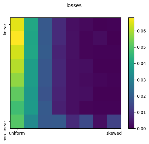 |
| Latent Interference (Minimum) | Clear separation from the non-linear regime, and increasing as linearity is introduced. | Same pattern, just slightly lower values. | The non-linear regimes allows the models to have these negative interferences without affecting performance. As the dimension increase the model can store the features with less interference. | 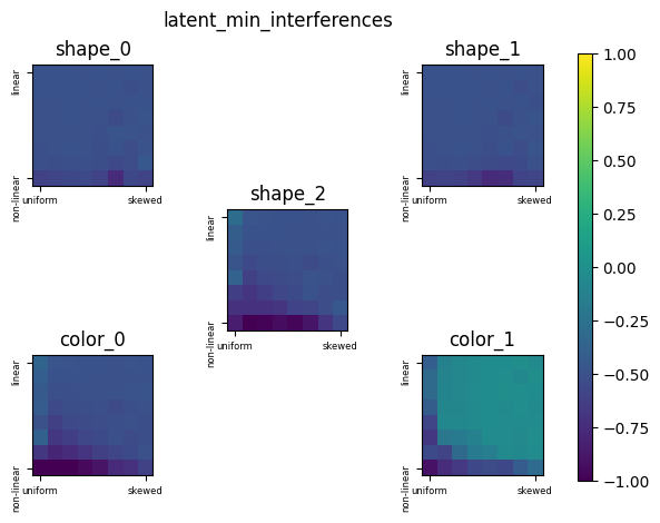 |
| Feature Interference (Unnormalized) | Consistently low and decreases as linearity increases. | Match the values of the normalized feature interference. | Features can collapse when there is insufficient space to accommodate them. Linearity effects the extent to which features collapse. | 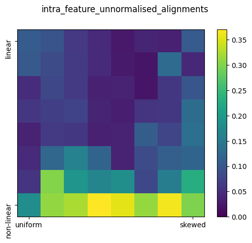 |
| Feature Interference (Normalized) | Consistently high. | There is a clear separation between the uniform and skewed distributions. Interference is lower for uniform distributions as the features are likely to co-occur and thus must be separated to limit interference. | The model actively distributes features according to the importance of the features, and not necessarily impacted by the linearity of the model. | 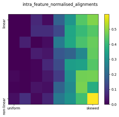 |
| Metric | Experiment Three | Experiment Four | Conclusion | Supporting Figure |
|---|---|---|---|---|
| Training Loss | Increases as linearity increases. There is a clear distinction between the two-dimensional models and the other models. | Relatively lower values but pattern is the same. | There is something significant about two-dimensions that means it is severely limited in representing five features compared to higher-dimensional models. | 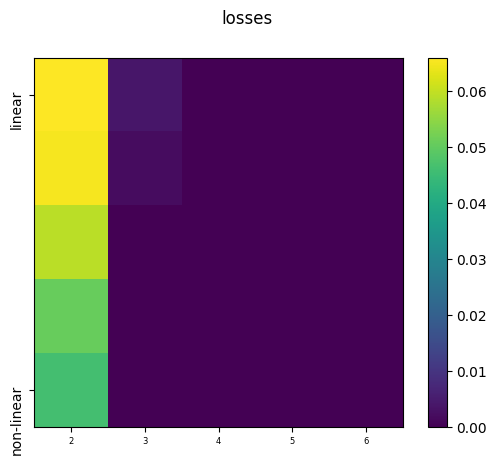 |
| Latent Interference (Minimum) | Highest for low-dimensional and non-linear models. | Same pattern. | Reflective of how the non-linearity allows the model to represent features with greater negative interference. Higher-dimensional models do not require this as they have more space to store features. | 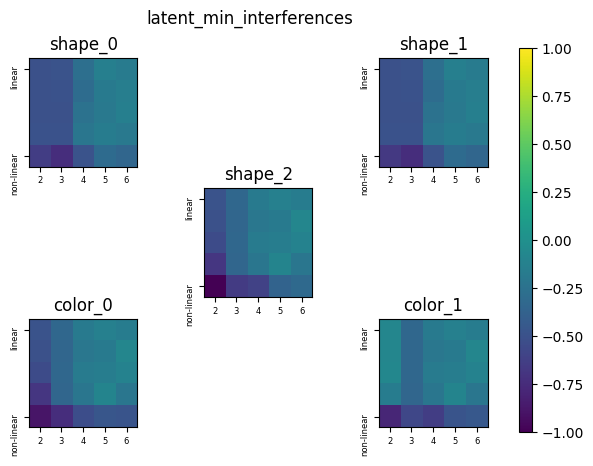 |
Generally what we observe is that there is a clear demarcation between models with two-latent dimensions and those with more latent dimensions. Similarly, there is a clear demarcation between fully non-linear model and those with small amounts of linearity. In particular, the effect of the linearity is most stark in the two-dimensional regime. This makes sense as in this regime the model is utilising superposition and thus putting more pressure on the non-linearity. However, as we increase the dimensions, the effect of changing the linearity on model performance is less pronounced, but it does promote different arrangements of the features.
InceptionV1
We now extrapolate these ideas beyond the toy model and to InceptionV1. We explore what happens to the InceptionV1 model when we intervene on its non-linearities.
Accuracy
We can try to understand the extent to which this model superimposes features by intervening on each of the blocks of the model. For each block we replace the ReLU activation with a leak ReLU activation of various parameters, and then test the performance of the model on a subset of the Imagenet-1K dataset. The intention is that if a block heavily relies on superposition, then intervening on it in this way will more negatively impact its performance.
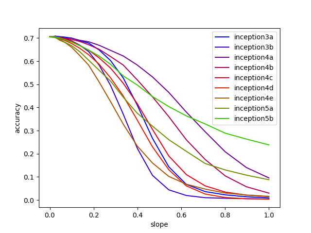
Interestingly what we see is that the inception3a and inception4e blocks are most significantly effected by these interventions, whereas the inception5b block is least effected.
- The inception3a block has the fewest number of neurons, so it would make sense that it holds more features in superposition. Moreover, the block is in the early part of the model, which has been identified to capture more textual features. Since textual features are usually more sparse than compositional, it make sense that the model utilises superposition here.
-
The inception4e block actually has a relatively large capacity, however, in other analyses it has been identified to have polysemantic neurons, see
Polysemantic Neurons in Zoom In: An Introduction to Circuits, suggesting that it is also reliant on superposition. - The inception5b block is the last block in the model and has 1024 neurons, which is more than the 1000 classes of Imagenet-1K. Therefore, since features are the most developed at this stage we would expect that they largely correspond to the individual classes, and thus the model does not need superposition as it can afford to assign features to orthogonal directions.
Prediction Collapse
For a model that stores features in superposition, removing the non-linearities would limit the model's capacity to retrieve those features, and would introduce interference between them. In particular, what we observe is that the model's predictions tend to collapse onto a few classes; potentially due to the fact that the interference at the intervened layer causes the activations of neurons to drop into negative territory such that at subsequent layers they are clipped and no longer contribute to the network's performance. Understanding how the predictions of classes collapse under these interventions can perhaps shed light into how features are distributed across neurons.
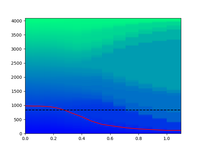
In this figure we give each class a colour, and plot a rectangle of height equal to the frequency with which it appears as a prediction across as sample of Imagenet-1K of size 4096. On the horizontal axis we have the parameter of the intervening leaky ReLU activation function. The dashed black line gives the number of neurons in the layer, in this case we are looking at the inception4e block which has 832 neurons, and the solid red line indicates the number of distinct class predictions made across the dataset. Clearly what we see is that the number of distinct predictions given by the model dramatically decreases, leaving only a few classes being regularly predicted. In this case they happened to be "buckle" which was predicted 1093 times, "mask" which was predicted 326 times, "chest" which was predicted 171 times amongst others. Therefore, we can conclude that features corresponding to these class are prominent across the neurons of this block.
This idea that the non-linearity helps retrieve the features in non-trivial ways to produce predictions is reinforced by observing the confidence with which the model makes its predictions at varying levels of intervention.
With no intervention the model expresses a wide-range of confidences due to the fact that some classes are very similar and so its cannot classify them with certainty. What the below figures show is the value of the logit corresponding to the actual class of the input and the logit of the class predicted by the model on that input.
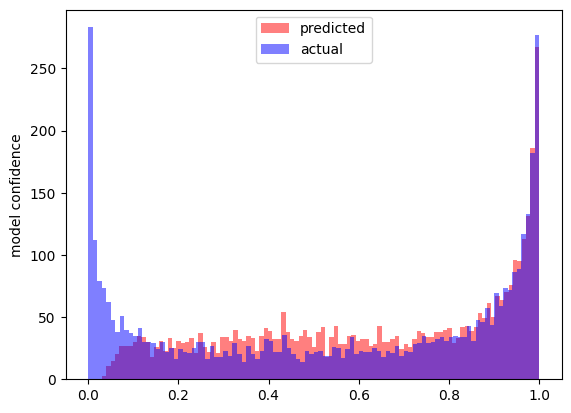
As we start to increase the slope of the negative component we see that the confidence with which the model makes its prediction gets gradually more skewed.
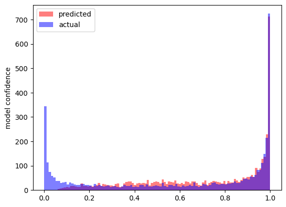
The above figure is with a negative slope of 0.0693. When we then consider a fully linear layer we observe that the predictions are very skewed.
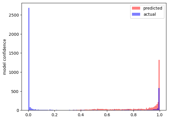
This is reflective of the fact that the model has fewer linearities to extract the nuance in the features. These figures were obtained from our intervention on the inception5b block.
Neuron Intervention
We can take this analysis further by intervening on specific neurons of the network. From Zoom In: An Introduction to Circuits, it was found that the 55th neuron from the inception4e block exhibited some polysemanticity; potentially because it is retrieving concepts from superposition. When intervening on this neuron specifically, we observe significant changes in the confidence with which the model makes its predictions.
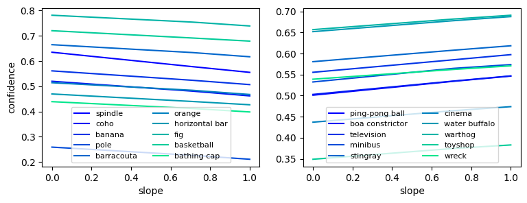
The above figure depicts the change in the average confidence given by the model to inputs labelled with the corresponding class as we intervene on the neuron; with the left plot showing the classes that experiences the largest drop in confidence and the right plot showing the classes that experiences the largest increase in confidence. Below are the result for the same experiment for a random neuron in the inception3a block.
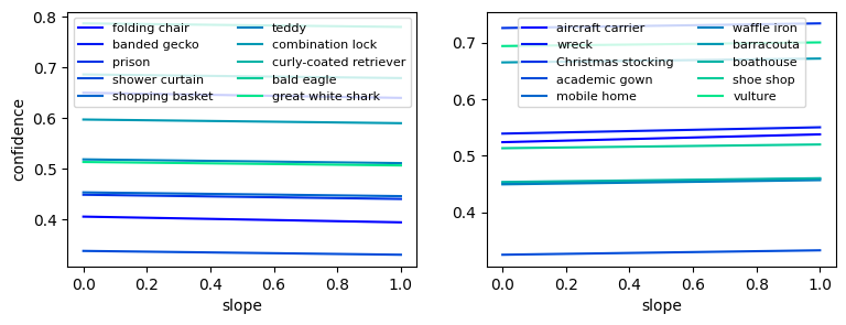
Clearly, the changes in this instance are not as significant, demonstrating that there is indeed something distinct about the 55th neuron of the inception4e block.
From Scratch
In the previous section we considered a model trained with ReLU activations and then explored its dependency on it by intervening on the layers. Here we instead train models with different activation functions from scratch.
We consider an autoencoder trained to reconstruct MNIST images, and a fully connected network to classify MNIST images as our testing grounds for ideas. In these settings, we can explore the necessity and rate of superposition by modifying various model parameters.
Reconstruction Task
Here our model architecture consists of an encoder and decoder component, and we test the effect of interventions when we train the model with leaky ReLU activation functions with different parameters at the intersection of these blocks. We measure performance by the mean squared reconstruction error.
The Effect of Latent Dimension
For a latent dimension $d$, the encoder architecture is $[784,128,64,d]$ and our decoder architecture is $[d,64,128,784]$. At the intersection of these blocks we apply the leaky ReLU activation function with parameters $\{0.0,0.1,0.4,0.6,0.9,1.0\}$. We consider latent dimensions $d\in\{8,16,32,64\}$ and train the models for 10 epochs on the MNIST train set. After training we then intervene by changing the parameter value of the leaky ReLU activation function and observe the subsequent reconstruction loss.
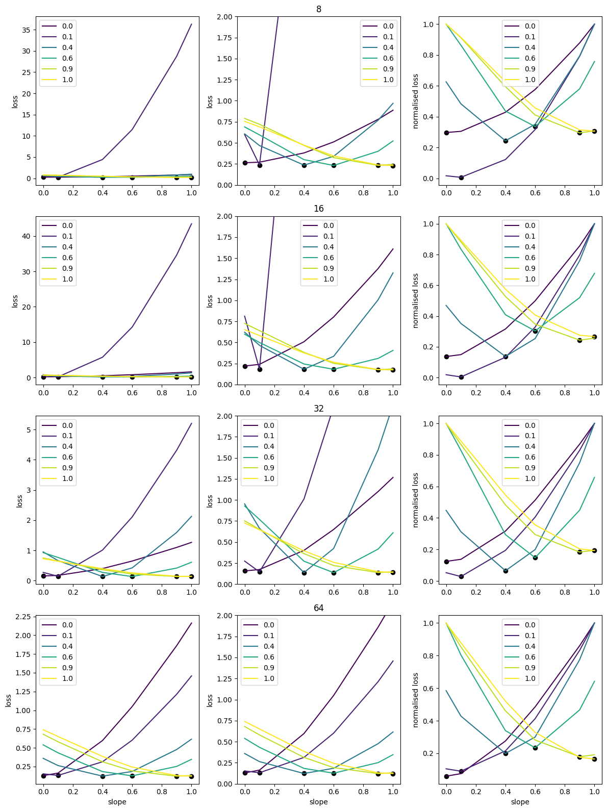
The rows of the figure correspond to architectures of varying latent dimension size. The left figures depict the reconstruction loss as we intervene on the activation functions, the middle figures are the same plot just with the y-axis capped at 2, and the right figures depict the normalised reconstruction loss. The black marker points on each line identify the slope with which the instance was trained, which also corresponds the colour of the lines.
From this we make the following observations.
- The reconstruction error can vary significantly as we intervene on the activation functions, suggesting that each model is relying to some extent on the non-linearity and representing features in superposition. Since the larger models appear to have a relatively flatter curve around the black marker, we could conclude that the larger models are less reliant on the non-linearity and hence are not utilising superposition as much.
- Each instance of the model is able to achieve relatively low reconstruction losses. In particular, the reconstruction losses appear to be fairly constant across every slope. Indicating that models can adapt their representations based on the amount of non-linearity they posses. Suggesting that superposition may be sufficient but not necessary for model performance. Furthermore, the right most figures indicate that the more linear models are more robust to subsequent interventions.
- As the model gets larger, the reconstruction loss introduced upon intervention gets smaller. Indicating that larger models are perhaps less reliant on the non-linearities for their performance, and can better distribute their representations.
- The performance of the fully-linear models is relatively consistent across model sizes. Perhaps indicating that the encoder block is only able to extract a few linear features to represent in the latent space. We test this hypothesis in the next section. Namely, if it were true then we would expect that increasing the size of the encoder block may be able to yield a lower reconstruction error in the linear setting.
From these observations we conclude that the non-linearity significantly affects the type of representation learned by the model.
The Effect of Encoder Size
Here, we fix the latent dimension of the autoencoder to $d=32$ and vary the layer sizes of the encoder block. More specifically, for $e=\{e_1,e_2\}\in\mathbb{N}^2$ we set the encoder block to have the architecture $\left[784,e_1,e_2,32\right]$. Training this model proceeds as before, however, we only consider the fully non-linear and linear regimes. We then test the reconstruction losses of these models using the same activation function that they were trained on.
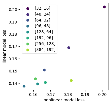
From the above figure we observe that as we increase the size of the encoder block the loss of the linear models decreases, as expected since now the encoder block is able to supply the latent space with linear features to represent. We observe that increasing the encoder size beyond a certain size doesn't yield better performance, on the contrary, performance starts to degrade. For these larger encoder sizes, it may be the case that they are too powerful, and providing the latent space too many linear features to represent which hinders performance; in this set up, the latent space can only store a maximum of 32 features independently.
Classification Task
MNIST
Here we train a feed-forward neural network on the MNIST classification task. We utilise an architecture of the form $[784,16,10]$, which we train with leaky ReLU activation functions with varying parameter values. Once we have this trained model we re-instantiate it leaky ReLU activation functions with different parameter values and observe the consequences on performance. The parameter values we consider are $\{0.0,0.05,0.15,0.25,0.4,0.6,0.75,0.9\}$.
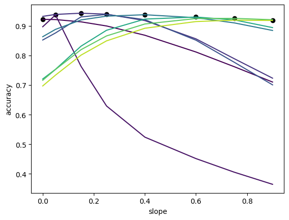
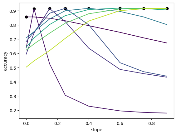
In the figure, each line corresponds to the accuracy of the model that was trained with leaky ReLU activation functions with parameter identified at the black scatter point.
What we observe is that generally this task is not too reliant on superposition, since accuracy does not vary too much on the interventions. In comparison to the reconstruction setting, where the loss varied significantly as we intervened on the activation functions. Suggesting that for this task the model is representing features compositionally rather than in superposition.
However, we do observe that training with some linearity improves the robustness of the model to these interventions, suggesting that it promotes less superposition in the model. This would suggest that to arrive at more interpretable models we should consider training with less
If we were now to consider a neural network with architecture $[784,8,10]$, we would expect their to be more superposition due to the lower dimensional latent space. Hence, we should observe that the effects of intervening on the activation functions is more significant. Indeed, this is exactly what we observe in the figure below.
Non-linear
The superposition hypothesis relies on the assumption that the latent representation of neural networks has some linear structure. In this case, features can be represented as directions and the purpose of the non-linearity is to extract those features to perform predictions. In our previous examples we have been intervening on layers where it is reasonable to assume that the representations have some linearity. For example, in the MNIST example, even though our network is dealing directly with the 784-dimensional image manifold, since it is very high-dimensional it is likely to exhibit some linear structure. In these cases, we intuited that the non-linearity allowed the neural network to store features in superposition, and thus we could control or identify the rate of superposition by intervening on the amount of non-linearity these function possessed.
However, now we want to explore what happens to our framework when this linearity in the latent representations is not present. For that we consider the task of classifying a sphere within a larger sphere with a hollow centre.
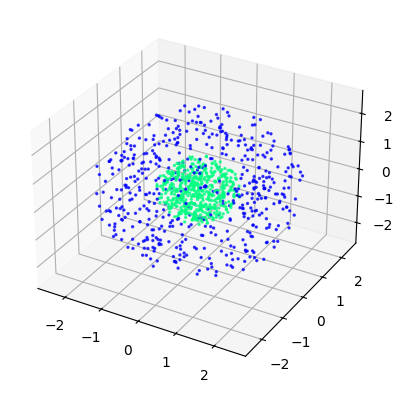
We repeat the procedure as in the case of MNIST, and we obtain the following results when considering a feed-forward neural network of architecture $[3,8,2]$.
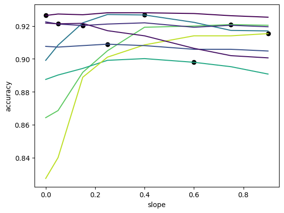
Where before we saw that performance translated relatively well across slopes, here we observe that it does not translate as well. Suggesting that the non-linearity in this instance is performing more complex operations that do not transfer well to activation functions with different amounts of non-linearity.
If instead we first pass the input data through a layer with a ReLU non-linearity, we improve the linearity of the representations and the interventions exhibit more predictable behaviour.
Conclusion
We first developed some intuition on how the non-linearities might effect a neural network's capacity to store features in their latent spaces. We then used this to empirically investigate how the non-linearity impacted the performance of a neural network. We validated some of our hypothesis with toy models, namely that the non-linearity plays an important role in superposition. We then extrapolated these ideas to explore the InceptionV1 models, and we observed how changing the non-linearity of a pre-trained model can cause its representations to collapse leading to a reduction in performance. We then focused on training models a priori with different amounts of non-linearity to observe how its performance would change when we then intervened on it. We observed that autoencoder models trained for reconstruction rely more on superposition, whereas, fully connected models for classification rely more on compositionality. Overall, we found that the activation function used significantly influenced the type of representation the model learned.
Reducing the amount of superposition in models is desirable to improve our ability to perform interpretability. Our observation that the amount of superposition is related to the amount of non-linearity may prove a viable path to controlling the amount of superposition in a model. Furthermore, these interventions on the linearity of the activation functions can be used to establish the amount of superposition in a pre-trained model; which may be useful for those performing mechanistic interpretability to identify potentially polysemantic neurons.
In future work it would be interesting to explore this idea further, by considering these interventions in more scenarios, and performing interpretability analyses on intervened models.