Feature Geometry
Features as Directions
There is a significant amount of evidence suggesting that large language models usually store features in their latent spaces using directions, a phenomena known as the linear representation hypothesis since it suggests that we can extract and manipulate the features using linear operations. Consequently, techniques such as dictionary learning using sparse autoencoders have been successful at extracting these features and subsequently manipulating the model's behaviour. Although the idea that models store their fundamental units of interpretations as directions is not so surprising from a statistical efficiency perspective, it is surprising that these features turn out to be interpretable. The emergence of interpretable directions was originally noticed in preliminary Word2Vec models, where the direction from the "king" to "queen" feature correlated with the direction from the "man" to "woman" direction.
To perform similar analyses for large language models one first has to identify the directions the model is using and to what features they correspond too. In the case of Wrod2Vec one could just use words to elicit the desired directions, however, large language models are more complex as they account for context. Sparse autoencoders surpassed this challenged by using sparsity as a proxy for unity. More specifically, it was hoped that by constructing an overcomplete sparse basis from which to construct the latent activations of these models, we would recover the features that the model was using to form its representations. It seems that so far this has largely been successful at constructing a dictionary of features that are relevant to the model's performance. With this we can start examining the geometry of these features to gauge the model's understanding. The first serious attempt at this to the directions from sparse autoencoders, identified algebraic structures, such as the "king"-to-"queen" and "man"-to-"woman" structure found in Word2Vec, and identified regions in the feature space that resembled similar constructions in the human brain.
Evaluating Feature Extraction
Here we try to take this analysis further by seeing if we can evaluate the performance of a sparse autoencoder by taking the linear representation hypothesis to the extreme. A priori there is no concrete way to evaluate the performance of a sparse autoencoder. Ideally, the sparse autoencoder would identify the exact set of features the model uses to form its representations. Note that these features may not be interpretable, in practice we see that a large proportion of them are, however, the model could just be utilising patterns that we are unaware of. Without a ground truth understanding of what the exact set of features, we cannot directly evaluate the dictionary learned by the sparse autoencoder.
Another hope we have for sparse autoencoder dictionary learning is that the features it extracts are interpretable. As mentioned before, this is achieved through a sparsity proxy, however, more sophisticated techniques have also been developed, such as $p$-annealing. Evaluating the sparse autoencoders in these instances is easier, as we often have an idea of what interpretable features are pertinent for the task. For instance, in the same work where $p$-annealing was introduced, they evaluate their resulting sparse autoencoders on models trained on chess and Othello transcripts.
However, here we return to the previous question of evaluating the sparse autoencoders capacity to retrieve the set of, not necessarily interpretable, features the model uses for its computations. To do this we make a fundamental assumption about the model developed by taking the features as directions hypothesis seriously. Namely, if the fundamental units the model uses to perform its computations are features stored as directions, then a sufficiently trained model should uniformly distribute these directions in its latent space, such to minimise the interference between features.
There are some challenges to this assumption.
- This may be the case for pretrained large language models, that are directly optimised for next-token prediction. However, as these models go through fine-tuning their internal representations may become skewed.
- The latent space of large language models are incredibly high dimensional, and so equally distributing these directions may be challenging or require a large amount of training.
- Large language models are probably unlikely to reach the global minimum of their loss functions, and so it may be the case that they can never reach this state by prolonging training.
With these challenges it may be unreasonable then to make this assumption. However, we can equally reverse this assumption and consider using it in a different way. Namely, we can use it to compare the different latent spaces of different models, or model layers. For example, if we suppose that the sparse autoencoders we train are roughly equally effective, then we can investigate the distribution of features for sparse autoencoders trained for different models or at different model layers to investigate their relative performances.
In this post we consider the set of sparse autoencoders provided by Gemma scope trained on the various residual stream layers of the Gemma 2 models. Since, these sparse autoencoders are trained in relatively similar ways we can assume that each are equally effectively at extracting the features of the model at their respective layers. Therefore, we can use them to evaluate the individual layers of the model by understanding how well they distribute their feature directions.
Results
The residual stream of the Gemma 2 2B pretrained model has $2304$ dimensions. Each sparse autoencoder learns a dictionary of size $16384$. We extract the $16384\times2304$ decoder weight matrix for each of the sparse autoencoders trained on one of 26 different layers, and we compute the cosine similarity of each feature by just multiplying this decoder weight matrix by its transpose and taking the strictly lower triangular matrix. We repeat this computation for a randomly drawn set of $16384$ features. We do this by drawing entries of a $16384\times2304$ from a random normal distribution and then normalising the columns so that the points are uniformly distributed on the unit sphere.
When considering these dot product we focus our attention on the distribution on the range $[-1,-0.1]\cup[0.1,1]$. We plot the histogram of these values for every fifth layer to yield the following plot.

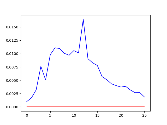
Clearly, the features extracted by the sparse autoencoders have heavier tails than the random features, suggesting that the features are clustered rather than spread out across the unit sphere. This is more starkly evidence when we depict the sizes of the tails as a proportion of the total distribution, with the red line representing the randomly drawn set of features.

Interestingly what we see is that for the initial and final layers the features are relatively well distributed, whereas toward the middle layers the features become more clustered.
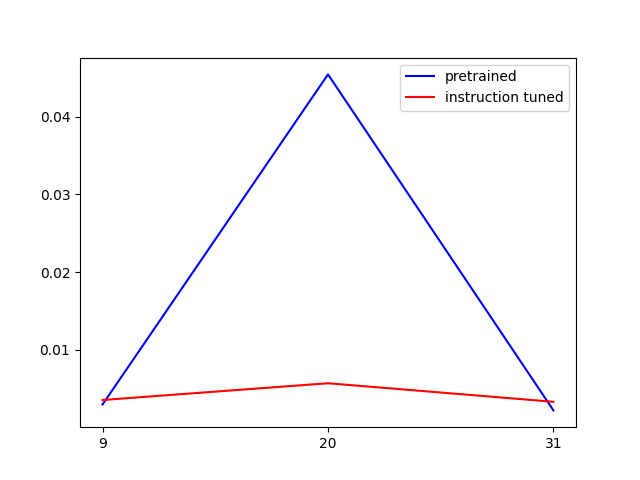
Recall that we postulated that fine-tuning would skew the distribution of the feature directions. We can test this by performing the same analysis but on the Gemma 2 9B model for which there are released SAEs for both the pretrained and instruction tuned models. In this case, sparse autoencoders for the pretrained and instruction tuned model are released for layers $9$, $20$, and $31$. As before, the dictionary size is $16384$, however now the dimension of the latent space is $3584$.

Interestingly, we see that for the earlier and later layers instruction tuning slightly decreases the uniformity of the features as predicted. However, for the middle layers it significantly improves the uniformity of the features.
Conclusions
Generally, what we see is that the directions learned by the sparse autoencoder are not uniformly distributed in the latent space of these models. Whether promoting such uniformity is a good idea would probably a good question to explore in future work. We do see that there is some correlation between the uniformity and the relative position of the latent space within the architecture of the model. At the middle stages, the model is probably combining lower level features into representations that can be then be used for high level extract in the later layers, meaning that there is some overlapping of features that results in the clustering of features in the middle layers. A more thorough investigation as to why features tend to cluster at the middle layers is perhaps warranted. Moreover, a more thorough investigating to the effects of fine-tuning on the uniformity of the features is probably worthwhile.